SHOCK AND DROP TESTING

A Shock test outputs a series of pulses to excite the structure under test. The response is measured at one or more locations on the structure and a spectral analysis is used to determine its response and resonance characteristics. This pulse response is an approximation of the impulse response, which requires a pulse of infinite amplitude. The Fourier transform of the impulse response is the Frequency Response Function (FRF) of the system.

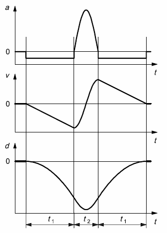
The Shock control process is essentially a time-domain waveform replication process that uses an FFT based algorithm to correct for the test system dynamics. The algorithm is similar to the one used for Random Control. The difference is in how the test profile is defined: in random control, it’s defined in the frequency domain; while in shock control, it’s defined in the time domain.

It is assumed that the test system is linear, which means that its response to any input can be predicted from its Frequency Response function. In the control process, this FRF is continually estimated and updated, and used to calculate the output drive signal. This output waveform should cause the test system to respond in a way that the control signal matches the test profile.

Figure 1: Mathematics of Control System

The system output y(t) can be calculated as the convolution between the system input, x(t), and the system impulse response, h(t).

y(t) = h(t) * x(t)

However, convolutions are tricky to calculate, and it may be impossible to fully determine the impulse response. Fortunately, this convolution is equivalent to a multiplication in the frequency domain. The system output y(t) is replaced with the output spectrum Y(f), the input x(t) is replaced with X(f), and the impulse response h(t) is replaced with the frequency response function H(f). Calculating the Fourier transforms Y(f) and X(f) are straightforward, and determining H(f) is much easier than h(f).

The controller calculates the required test system input x(t) by:

x(t) = IFFT( X(f) ) = IFFT( R(f)/H(f) )

= IFFT( FFT( r(t) ) / H(f) )

where R(f) is the test profile in the frequency domain and IFFT is the inverse FFT (an algorithm for the Fourier transform). The test profile is specified by the user as r(t), in the time domain, and is then transformed into R(f) before the test begins.

In the classic shock test, r(t) can be a half-sine, sawtooth, triangle, rectangle, trapezoid, or haver-sine shape.

The target pulse shape can be half-sine, sawtooth, triangle, rectangle, trapezoid, or haver-sine. The pulse itself is always one-sided — its displacement is only in one direction. A series of these pulses would cause an unbounded armature excursion of the shaker in one direction, which is not physically possible. To keep the armature centered, each pulse must have a zero mean displacement. This is done by adding a compensating pre- and post-tail to the pulse.

Waveform Compensation In Shock Testing

At the end of each pulse output, the shaker must return to its rest position. However, the pulse shapes used in the classical shock test are one-sided, meaning that, if used by themselves, they would leave the shaker armature with residual displacement and velocity. A series of these pulses would cause the armature to travel all the way to its stops, and then no more outputs would be possible.

Compensation is the method of “correcting” the control signal so that the ending displacement and velocity is always zero. It involves adding smaller pulses before and after the main pulse.

Figure 2: A single square pulse and its effects on velocity and displacement over time

Given a main pulse shape, there are different algorithms that can be used to generate an optimized waveform. Compensation pulses can be added before or after the main pulse.

The figure below shows a half-sine pulse that has been properly compensated, along with its velocity and displacement profile.

Figure 3: Shock pulse compensation

When generating the profile waveform, it is important not to exceed the limits of the shaker. These limits include the voltage and current capabilities of the power supply driving the system, and the ability of the system to generate peak acceleration, force, velocity, and displacement levels.

Recommended for Shock Tests

Spider-81: Fourth generation vibration controller with Classic Shock test software option.