With various excitations, the characteristics of the UUT system are measured experimentally. These characteristics include:
- Frequency Response Function (FRF), which is described by:
- Gain as a function of frequency
- Phase as a function of frequency
- Resonant Frequencies
- Damping factors
- Total Harmonic Distortion
- Non-linearity
Frequency response is measured using the FFT, cross power spectral method with broadband random excitation. Broadband excitation can be a true random noise signal with Gaussian distribution, or a pseudo-random signal of which the amplitude distribution can be defined by the user. The term broadband may be misleading, as a well implemented random excitation signal should be frequency band-limited and controlled by the upper limit of the analysis frequency range. That is, the excitation should not excite frequencies above that which can be measured by the instrument. The random generator will only generate random signals up to the analysis frequency range. This will also concentrate the excitation energy on the useful frequency range.
The advantage of using broadband random excitation is that it can excite the whole frequency range in a short period of time so the total testing time is less. The drawback of broadband excitation is that its frequency content is spread over a wide range within a short duration. The energy contribution of the excitation at each frequency point will be much less than the total signal energy (roughly, it is -30 to -50dB less than the total). Even with a large average number for the Frequency Response Function (FRF) estimation, the broadband signal will not effectively measure the extreme dynamic characteristics of the UUT.
Swept sine measurements, on the other hand, optimizes the measurement at each frequency point. Since the excitation is a sine wave, all of its energy is concentrated at a single frequency, eliminating the dynamic range penalty in a broadband excitation. In addition, if the frequency response magnitude drops, the tracking filter of the response can help to pick up extremely small sine signals. Simply optimizing the input range at each frequency can extend the dynamic range of the measurement to beyond 150 dB.
Measure the Frequency Response Function using Swept Sine
A sine signal with a fixed frequency is expressed in the following Frequency Response Function formula as:
where t represents time. A sweeping sine signal has a changing frequency that is usually bound by two limits. The frequency change can be either in the linear scale or logarithmic scale based on different user requirements. The swept sine signal can be defined by the following parameters:
- The low frequency boundary, which is simply called Low Frequency or
- The high frequency boundary, which is simply called High Frequency or
- The sweeping mode, either logarithmic or linear
- The sweeping speed, in either octave/min if the sweep mode is logarithmic, or in Hz/Sec if the sweeping mode is linear
- The amplitude of the sine signal, A(f, t), which can be a constant or a variable of time and frequency.
The instantaneous frequency represents the current frequency of the sweeping sine. It is a changing variable and usually displayed on the screen as Sweeping Frequency
The Sweeping frequency can also be manually controlled during the test with the Hold, Resume, Jump or Pause controls.
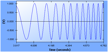
Unlike some Digital Signal Analysis (DSA) products which use swept sine test with multiple discrete stepped sine tones in a sequence, the CI swept sine test uses a true digital synthesizing technique to generate sine sweeps with extreme analog-like smooth transition from one frequency to another. This ensures that there are no sharp transitions during the test that might ¡°shock¡± the UUT. The picture below shows a typical swept sine signal with 1.0 Vpk.